Advanced Properties of AC Circuit (25th Day)

Spring 2015
Professor Mason
June 2 Class

Formulas used in AC circuit experiment

The first thing we did in class was about reviewing the formulas and equations that we were going to use for the rest of the class including [Xc = 1/wC], [Xl = wL], [Vrms = Irms Z], [z = sqrt of R^2 + (Xl - Xc)^2. Moreover, if the Xl is zero, the circuit becomes like the one drawn in the picture attached on the left, which has an equation of [z = sqrt of R^2 + Xc^2]; therefore, we can say that [Vrms = (sqrt of R^2 + Xc^2) Irms]. As shown in the picture attached on the left, we can also say that [Irms = Vmax/ (sqrt 2) (sqrt R^2 + (1/wC)^2)]. In class, professor asked us what would happen to Irms if the frequency is doubled; the answer to that question is the Irms would be four times bigger because of the equation [w = 2 pi f] and [Xc = 1/wC].


















Circuit experiment on Logger Pro

 In class, we needed to do an experiment about AC circuit, and we were given things, such as 100 uF Capacitor, 10 Ohm resistor, Function generator set at 10Hz and 1000Hz, and motion detector set on logger pro. We first needed to do the 10Hz frequency set on function generator; next, we needed to do the 1000Hz frequency set on function generator. We also set 1V as the voltage max on the function generator. The setup is shown in the picture attached above; while the graph of Current vs time and Voltage vs time shown in the picture attached below. We needed to attach the current censor series to function generator and capacitor, and we also needed to attach the voltage probe to the function generator for both positive and negative charges. We needed to set the first one on 5000 samples and measured for 0.5 seconds; the maximum samples we could do was 5000 samples only because we set up 2 censors (voltage probe and current censors) at the same time in order to make the graph looks more smoother (not sharp).

 We still needed to do the next experiment, which was dealing with 1000 Hz frequency set on function generator. For this one, we needed to set the data samples on 0.01 seconds with 50000 samples in order to make the graphs look smoother instead of sharp looking graph. This time, we could set the data samples on 50000 samples because we only had 1 censor at a time, and it must be attached to CH1 on the motion detector, otherwise, it would not work. We needed to use only 1 censor at a time because if we used two censors instead, we could only collect 5000 samples, which would not produce a smooth graph on Logger Pro. The Voltage vs time graph is shown on the picture attached above; the current vs time graph is shown in the picture attached below.

After we finished with the experiment, we needed to measure the experimental Vmax, Imax, Vrms, and Irms as well as theoretical impedance, Vrms, and Irms. This time, we could use multi meter in order to measure the experimental Irms and Vrms on the circuit.

Experiment and Calculations on 10 Hz and 100 Hz frequencies

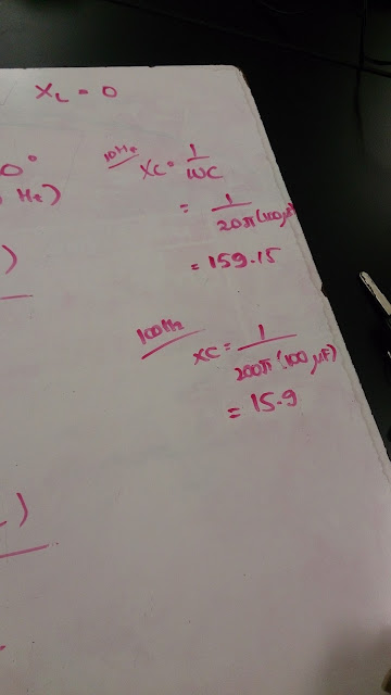
 Next, we had to do another experiment, but the differences were the frequencies we used. For this experiment, we had to use 10 Hz for the first experiment, then 100 Hz experiment for the next one. After were done setting all up on the Logger Pro, we needed to measure the experimental phase difference by measuring the difference of times between the Max current graph and Max voltage graph divided by the period, which has an equation of [T = 1/f] on Logger Pro. The phase angle has an equation of [Phase angle = Phase diff * 360 degree]; we needed to do both for 10 Hz and 100 Hz frequencies in order to get the experimental calculations. The answers are shown in the pictures attached on the top left, and middle left.

 After we finished with the experimental calculations, we moved on to theoretical calculations. Theoretical calculations have an equation of [Phase angle = tan (theta) = (Xl - Xc)/R] by using the calculations calculated above. After we finished doing the calculations and experiments for phase difference and phase angle, we continued on doing resonance in RLC circuits. In class, professor showed us the graph of I that becomes Imax when Xc = Xl shown in the picture attached on the left; the top one is called the resonance peak. We were provided a formula for this kind of problem, which is [fo = 1/ 2pi(sqrtLC)], which fo is the resonance frequency.

 Next, we needed to predict a circuit based on what the professor said in class and drew it on the board; it is shown in the picture attached on the left. In this calculation, we first needed to find the f based on Imax using the given formula on the above; then, we needed to calculate the power average, which has an equation of [Pavg = 1/2 (z I^2max cos(theta))], which cos(theta) here is defined as power factor. The works are shown in the picture attached on the left.

 Based on the predicted circuit as shown in the picture attached before, the setup of the real circuit is shown in the picture attached above. Then, we needed to find for the right or maximum frequencies  with multi meter and function generator.

 The steps for this experiments are: set everything up in series, watch current in multi meter, tweak the frequency in function generator, find the range where the current reach its peak on multi meter, get the average of the frequencies, and finally, the obtained value is the resonance frequency shown in the function generator. Therefore, we basically were looking for the right frequency based on the measured current in multi meter.

Voltage and Current in AC Circuit (24th Day)

Spring 2015

Professor Mason

Physics 4B

May 28 Class

Graph and Properties of AC Circuit

The first thing we learned in class was about the properties of AC circuit, as well as the Voltage vs Time graph and Current vs Time graph. In class, professor Mason showed us the form of Voltage vs Time graph in AC circuit, and it is shown in the picture attached on the left; he also showed us the form of Current vs Time graph in AC circuit; the difference between those two graphs is that Voltage vs Time graph has higher amplitude than Current vs Time graph (NOTE: the graph in the picture on the left is wrong, the top one should be I vs t, and the lower one should be V vs t because V vs t graph has higher amplitude than I vs t graph; they should be swapped). We also learned the properties of AC circuit in class, and one of those is the Voltage across resistors, which has an equation of [V = Vmax Sin(2 pi f t)] or [V = Vmax Sin(wt+flux) + Vo], and [w = 2 pi f = 2 pi/T]. We also found out an equation of current across resistors, which is [I = Imax Sin(wt + flux) - Io]. Professor told us an average value of V vs t graph (sin graph) is equal to zero; however, if this sin graph was squared, the graph becomes like the graph shown in the picture attached on the left [V=Vmax sin (2 pi/T)t]. The average value of sin squared equation is equal to cos squared equation value. We also found out that Irms and Vrms has equations of [Irms = Imax/2^1/2] and [Vrms = Vmax/2^1/2]. In class, we also learned that Average Power has an equation of [Pavg = 1/2 I^2max R], so that [Vrms = Irms R]. 

RMS and AC Current and Voltage Experiment

 After we finished learning the properties of AC Circuit in class, we continued to the experiment. This experiment's setup contains current sensor parallel to a 100 Ohm resistor, Voltage probe, function generator, and motion detector connected to logger pro. We first needed to set the frequency and voltage in function generator to 10 Hz and 3 V.

The pictures attached on the left shows how we set up the circuit, and the graph picture on the left shows us how the Current vs Time and Voltage vs Time graph would look like after we hit "Collect" button on Logger Pro based on our circuit setup. Next, we needed to find the Vmax and Imax from the graph to calculate the experimented Vrms and Irms.

After we got the graph, we needed to compare the theoretical Vrms and Irms measured from the multi meter with the experimented Vrms and Irms from the graph. They turned out to be almost the same, and the percent error turned out to be 36.4% for Irms and 1.45 % for Vrms shown in the picture attached on the right.

After we finished the experiment, we figured out a new equation, which was [Q = Integral of I dt], which would equal to [I = C dv/dt]. Based on this experiment, we also found out that Current as a function of time across capacitor has an equation of [I(t) = C Vmax w cos(wt+flux)]. The difference in amplitude in graph from V has a difference by I(t) = C w.



Capacitive and Inductive Reactance

 After we finished the calculation based on the experiment above, we continued to phase difference and Capacitive reactance and Inductive Reactance. We were given an equation of phase difference, which is [Phase diff = delta t/T], which would be used later on the next experiment. We also found out an equation of capacitive reactance, which is [Xc = 1/ cw] or [Xc = 1/2 pi f c], and also can be [Xc = Vrms/Irms], which Xc has a unit of Ohm. On the other hand, inductive reactance has an equation of [Xl = wL] or [Xl = 2 pi f L].

Experiment with 100 uF capacitor

 In this experiment, we had the exact setup and steps as the experiment with 100 Ohm resistors; the only difference is we were using 100 uF capacitor instead of resistor. The picture on the left shows us how we set up the circuit for this experiment. After we hit "Collect" button, it would show up a graph like shown in the picture on the left. The calculated Vmax, Imax, Experimented Vrms and Irms, Theoretical Vrms and Irms are shown in the picture attached below, as well as the percent error.

 This time, we needed to find the phase difference, which is the time difference between v vs t graph reach first max point and I vs t graph reach first max point divided by period; we got 0.24 as the phase difference.

Experiment with Coil

This last experiment today was also the same as the other two experiments; however, the only difference is we used coil instead of resistor of capacitor. This time, we needed to compare this result with the previous result on previous meeting. The graph looks like this, shown in the picture attached above, when it is connected to motion detector, function generator, and probe in Logger Pro.

Phase Angle and Impedance

The last thing we learned from today's class was the formula of phase angle and impedance. Phase angle has an equation of [tan (theta) = Xl - Xc/R], while impedance has an equation of [Z = square root of R^2 + (Xl - Xc)^2], which theta is the angle for phase angle, and Z is the impedance. 

Inductance in DC Circuit (23rd Day)

Spring 2015
Professor Mason
Phys 4b
May 26 Class

Inductor Voltage and Current
The first thing in class that we learned was about Inductor Voltage and Current. An inductor is a coil of wire which stores energy in a magnetic field when it carries a current. The inductance L of an inductor is defined as the magnetic flux through the inductor per unit current. Then, we were given an equation of [L = Flux max/ i]. Any change in the current through an inductor leads to a change in the magnetic field it produces. It also will lead to a change in the magnetic flux through the inductor which, produces in induced emf in the inductor according to Faraday's Law. In the lab manual, we were given a graph of potential difference across the inductor after the switch is closed, and the voltage vs time graph is shown in the picture attached below.

The graph were measured by a tool shown in the picture above. 

The moment the switch in a circuit is closed, there is no current flowing, and the voltage across the inductor is the same as the emf of the voltage source. The current starts to increase from zero, and it changes rapidly at first, and it also levels off as it reaches its steady-state value of [epsilon/R]. The potential difference across the inductor decays exponentially with the rate of change of the current as provided with an equation of [VL = E exp(-t/Time constant)], which Time constant has a formula of [Time constant = L/R] (only applies for DC circuit). The current vs time graph is shown in the picture attached below.

This picture attached above also shows us that 100 ohm resistor has the colors of Brown-Black-Brown line on it. We were also asked to calculate the value of induction of the coil if the coil has an area of 5 by 5 centimeters and also has a length of 5 cm; we calculated it using an equation of [L = Uo N^2 A/Lo], which is shown in the picture above as 4.9x10^-2 H as the answer for that calculation. We were also asked to find the value of resistance based on a copper coil of 18H (gauge) using an equation of [R = rho L/A], which is shown in the picture above as 0.3 ohm as the answer of that calculation. 

Oscilloscope Experiment

Next in class, we needed to do an experiment on oscilloscope attached to a coil and a resistor in order to find the right current function graph. The steps to set up the oscilloscope are: 1. connect alligator clip from CH 1 across the output of the function generator, 2. set the function generator to produce a sinusoidal wave form, 3. set the triggering source to CH1, 4. Trigger on a positive slope, 5. adjust horizontal, vertical scale, position knobs, and triggering level knob, so it has a stable display of graph. The sketch of the circuit we needed in this experiment is shown in the picture below. 

In this experiment, we needed to set up a circuit attached to an oscilloscope, and the steps are as follows: 1. measure the resistance Rl of the solenoid and R of the resistor with the DMM, 2. construct the circuit as shown above assuming that the internal resistance r of the function generator is 50 ohm, 3. connect oscilloscope in parallel with the solenoid, 4. set the function generator to produce a square wave form, 5. adjust vertical and horizontal scales and positions of the oscilloscope to display the voltage across the inductor, 6. adjust frequency of the function generator, 7. measure the half-time t_1/2 of the decay of the induced emf in the solenoid, 8. determine the inductance of the coil and its uncertainty from the measurement, 9. use measured inductance to determine the number of turns N in the solenoid and uncertainty. The graph shown in the oscilloscope based on the circuit above is shown in the picture attached below.

 The picture attached below shows us how we set up the function generator, oscilloscope, resistor, and inductor(coil) based on the sketch of circuit given from the lab manual.

The calculation part of this experiment is all shown in the first picture attached at the very top of this blog; we needed to use the total R of 150 ohm because of the 100 ohm resistor added by the internal resistance of the function generator, which is 50 ohm. Then, we needed to find the period and the frequency, and they are all shown in the firs picture attached on this blog. 

The picture attached above shows us the percent error for the resistor, which is 5%; it also shows us the uncertainty for t_1/2, which is plus minus 2x10^-7 s.

Faraday's Law of Induction

Next, after we finished the oscilloscope experiment session, we continued to doing calculations on Faraday's Law of induction, which has an equation of [E = (-d Flux B/dt)N]. We were given a circuit as shown in the picture attached above, and first, we needed to calculate the time constant that has a unit of seconds shown in the picture above. Then, we also needed to calculate the voltage drop across the resistors, calculate how much time it takes from the voltage drop to exactly 11 V, calculate how much energy dissipated, calculate how much energy stored on the whiteboard using the formulas shown in the picture attached above. 

Ampere's Law, Coil, and Solenoid (22nd Day).

Spring 2015
Professor Mason
May 19 Class


Computer  Work (13.9 and 13.10)
In class, we were given several works to do on the computer. First, we had to type "active physics" on Google, then click on "University Physics," which has a link: (http://wps.aw.com/aw_young_physics_11/). We first need to pick part IV Electromagnetism; to do that, we need to click the bar at the top left corner and switch it to electromagnetism. First, we had to do 13.9, which is the electromagnetic induction. This picture attached below shows us the questions provided on section 13.9 as well as the magnetic flux simulation to play with in order to help us finish all the questions.

The answers for each question on section 13.9 are shown in the picture attached below.

In the beginning of class, we also were given some equations of [E = d(flux . B)/dt], [Flux B = Integral of B vector dA or Integral of B vector cos(theta) dA], and the last one was [E = -N(d Flux/dt or E = -N(d BA cos(theta)/dt)]. While we were doing this computer work, professor Mason showed us an experiment with big magnet and rod. The diagram of where the magnetic field and the force of the rod is going is shown in the picture above; the experiment is shown in the picture attached below. 

With the power supply attached to the experiment tool, we could set up the rod as much as we wanted to; for example, we could either make the rod move towards the big magnet or make the rod move away from the big magnet depending on how the professor set the power supply. 

After we finished computer work section 13.9, we continued on doing section 13.10, which is shown in the picture attached below. 

 The picture above shows a Motional EMF simulation for section 13.10, which is the Motional EMF; as well as the simulation in section 13.9, we could play with this simulation as well, such as adjusting the length, resistance, magnetic field, and velocity; we could also choose which graph would it provide for us (I E and flux).

 The answers for section 13.10 are shown in the picture attached above, except for question 13; question 13's answer is shown in the picture attached below. Based on the picture above, we found out an equation of [Induction I = -BLV/R].

Inductions Properties

 In this class section, we learned some things about inductions and inductor; one thing we found out about inductors is that inductors function like capacitors, but it stores energy by the magnetic field. We also learned that as V increases, I decreases; as B increases, back emf also increases; as number of coils increases, R also increases; finally, the bigger the coil, the bigger the resistance is.

 We also found out some new equations, and one of them is [C = Q/V = I(dB/dt)/V]; that equation comes from the three equations of Voltage, which are [V = L(dI/dt)], [V=IR], and [V = I(dB/dt)/C]. We were also given an equation for B solenoid, which is [B solenoid = Vo I (N/L)].

In the middle of the class, we were asked to do some calculations for induction of coil; therefore, we needed to use an induction of coil formula, which is [L = Uo N^2 A/ Lo (dI/dt)], which Uo is a constant of 1.25x10^-6, and L has a unit called "Henry." We also learned that there are ways to decrease and increase inductions in coil. Ways to decrease inductions are: 1. Reduce the distance of plates, and 2. put something in between the plates; ways to increase inductions are: 1. increase the area of plates, 2. increase the length, 3. increase the loop, and 4. increase the Uo permibility (insulator). Based on the picture attached above, we learned that inductor acts like nothing in a wire or coil (dI/dt = 0). 

Another Computer Work (14.1)

After we finished doing some calculations on inductions, we continued on doing the computer work section 14.1, which is the RL circuit. Similar to section 13.9 and 13.10, this section 14.1 also has a simulation called RL circuit simulation to play with. This time, we can adjust the R, L, and V in order to help us finish all the question through this section. The simulation is shown in the picture attached below. 

 The answers for section 14.1 are shown in the picture attached above.

For question #2, we took a picture of the answers on computer because we need the detailed answer, and it is shown in the picture attached above. For this questions, we learned that Faraday's Law states that if the magnetic flux through a region of space changes, an electromotive force, or EMF, is induced in the region. The direction of the induced EMF is such that if charge is present in the region, the EMF will drive the charge to create magnetic flux in opposition to the original change in magnetic flux. The magnitude of the induced EMF is proportional to the rrate of change of magnetic flux. 

For question #8, this is how we got 1.7 A through some calculations, and it is shown in the picture attached above. Based on this computer work section 14.1, we learned that if we double the inductance, the time increases, and if we double the resistance, the time decreases. Based on this work, we also learned that Time constant is perpendicular to 1/L; if Time constant equals to 0, it means that it is going slow; if Time constant equals to infinity, it means that it is going fast. In conclusion for this work, the formula we need to know is [Time constant = L/R].