Magnetic Loop (20th Day)

Spring 2015

Professor Mason

May 12 Class

Magnetized Pin

In class, we had to draw the magnetic field of an ordinary pin and magnetized pin, and this picture attached below shows us that ordinary pin has positive and negative charges arranged randomly close to each other; while the magnetized pin has separated positive and negative charges inside the pin.

Based on the professor's lecture, we found out that when there is magnetic field, there will exist force; magnetic force is defined as an equation of [F = IL x B vector] and torque as an equation of [T = IL^2B]; thus, we could also say that [F = qv x B vector].

In class, we also learned that there are two ways to destroy magnetism in an object, and those are by heating up the object until it reaches certain temperature, and by hitting the object with a hammer. In class, the professor did an experiment with a magnetized pin; he showed us how to eliminate the magnetism in the pin by heating it up with a blowtorch shown in the picture attached below. The second way is to hit the object with a hammer; hitting the object with a hammer will cause a massive vibration to that object and will eventually lose all the magnet inside the object. 

Magnetic Loop and Torque
In class, we had to do a calculation to find the net force of a current loop and to find net torque acting on the loop. We found out that the definition of torque is R x F; we also found out the bigger loop has bigger torque.

The picture attached above shows us the calculation to find the torque of a loop and the direction of the loop. We used another equation of [T = NIAB] to find the torque. The calculations are shown in the picture above. For the direction of the loop, it would be 90 degrees because A is perpendicular to I. For the calculation shown in the picture below, we also used an equation of [T = NIAB].

Experiment with Magnet and Power Supply

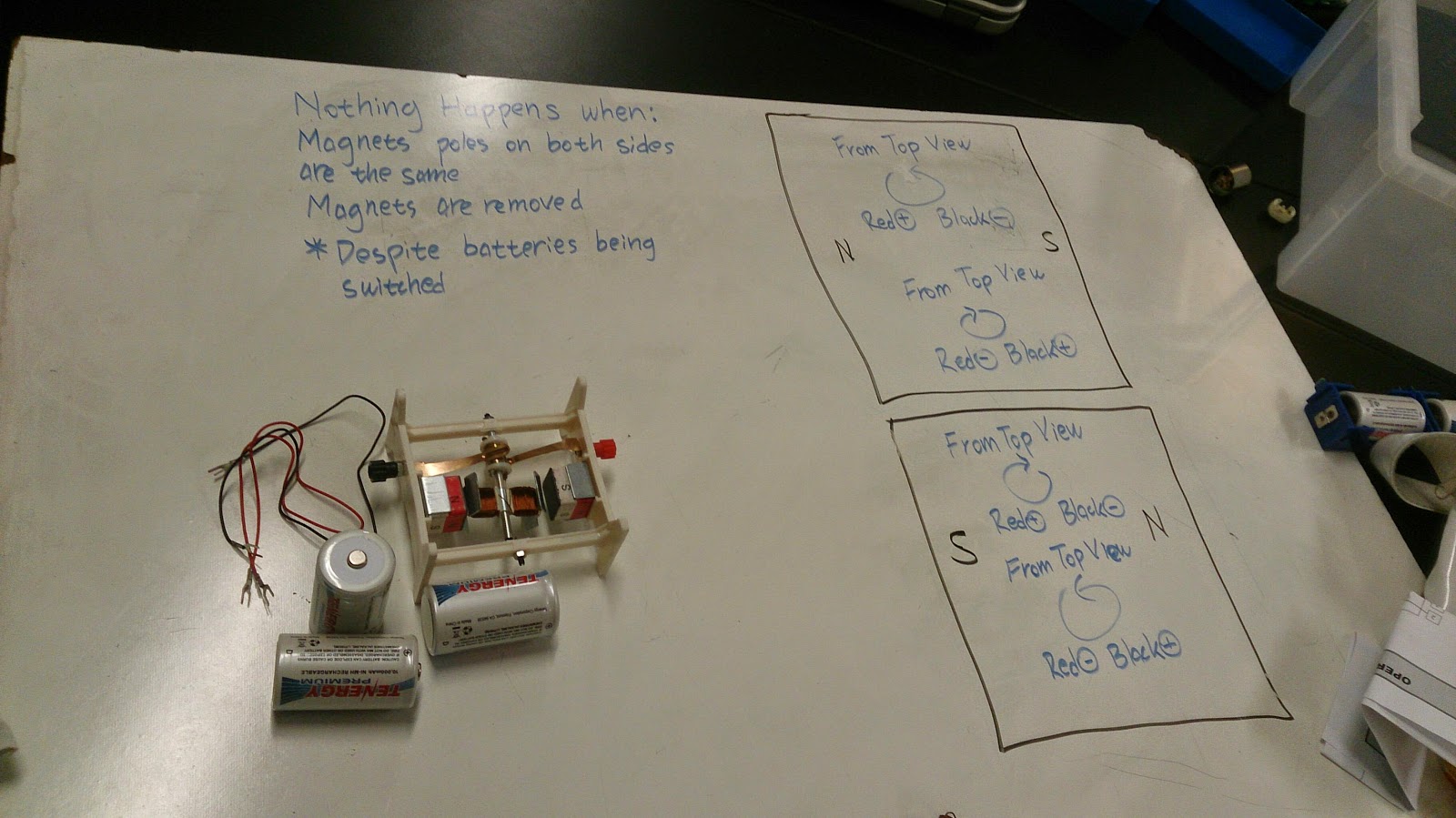
In class, the professor told us that the things that most likely would make a motor to fail to work are brush, coil, and commuter. Then, we continued doing to the experiment, which involved this thing shown in the picture below. 

We needed three batteries and wire attached to this thing in order to get it working. However, before attaching all the stuff needed, we also needed to adjust the direction of the magnet. After all things had been set up, we attached the wires to the batteries in order to make the thing in the middle with copper spun; the direction of where the thing would spin depends on the direction of the magnet (North and South).

We need to determine the direction of the spin based on the magnet. First, we did North-facing magnet on the left and South-facing magnet on the right. The result is shown in the picture attached below. On the other hand, we also needed to do the other way around, which South-facing magnet would be on the left and North-facing magnet on the right. Also, nothing happened when the magnet poles on both sides are the same (North facing North and South facing South). The magnetism in this thing cancelled each other out when they are facing the same sides. 

The next experiment we did was to make the circular copper wire spin. The things we needed for this setup was a power supply, alligator clips, magnetic bar, circular copper wire, and two copper wire holders to keep the copper wire from falling. First, in order to get it working, we needed to attach the alligator clips to the power supply, and set it to 4.5 Volts; after the set up was completed, the circular copper wire would spin as shown in the picture attached below. Before the setup was completed, we had to rub one end of the copper wire with sandpaper 360 degree; for the other end of the wire, we just needed to rub it 180 degree with sandpaper; we had to do this in order to connect the wire with the power supply.

Experiment with Magnetic Pole

In this experiment, the professor put a magnetic pole in the middle, and he placed 5 compasses around the magnetic pole to see which direction the compasses are pointing. 

As shown in the picture attached below, the compasses are pointing in circular motion. The directions of the compasses depend on the flow of the current; therefore, by reversing the current flow, it reverses the direction of the compasses as well. Finally, we could conclude that B vector is perpendicular to the current, and B vector is also perpendicular to 1/r, which r is the distance from magnet to compass. 

Loop Calculation

This time, we were given a setup of a loop, and we needed to find the dB, which dB has a definition in a form of equation of [dB = (Uo/4pi) (IdI x r vector/ r^2)]. 

In this problem, we also found out a new equation, and that is [Fb/Fe = Eo Uo V^2], which could be simplified as [Fb/Fe = V^2/C^2]. In this calculation, we were given that Uo and Eo are constants, which are [Uo = 1.25x10^-6] and [Eo = 8.85x10^-12]. The complete calculations are shown in the picture attached below. 

Magnetic Properties (19th Day)

Spring 2015
Professor Mason
May 7 Class

Magnetic Field Sketch
In class, the first thing we needed to do was to draw the magnetic field using arrow around the magnet. We were given a random magnet, then we placed it on the white board. We had to determine the the direction of the arrow by using compass; the arrow points toward the north direction of the compass. After we finished the experiment, we found out that our magnet had two magnetic field, and the main point of the field was placed in the middle of the magnet as shown in the picture attached. Therefore, when we drew a continuous arrow, it would look like a butterfly.

Flux and Gauss Law Magnetism Proof
In class, we were asked to create a flux sketch based on our magnet; however, out magnet had a weird magnetic field, so we changed it to a normal magnet with normal magnetic field. Flux is defined as net number of poles enclosed divided by epsilon, [Flux = N/Eo], which would always be equal to zero. We also found out the unit of magnetic filed (B vector) is Tesla or Gauss; 1 Gauss is equal to 1/1000 Tesla. We had an interesting experiment involving magnet; first, we had a magnetized paper clip, then we cut it in half, and the result is each clip now has different pole. This also applies for the big magnet as shown in the picture above. If we break the magnet, it still has pole going on through the big magnet.



Magnetic Force
In class, we learned that most field, such as gravitational field and electric field, are part of force field; therefore, Magnetic Field is also a force field. Force of the magnetic field is perpendicular to electric field; the fun fact is that magnetic field also exists inside our brain. +Ve charge rotate clockwise, -Ve charge rotate counterclockwise. For electrons, we use left hand rule, and for protons, we use right hand rule. Magnetic force is defined as an equation of [F = qv x B], which B has a unit of kg/CS.

Magnet and Oscilloscope
We had an experiment in class, which it involved with an oscilloscope. We put a big magnet on top of the oscilloscope, then the graph on the oscilloscope changes. We also needed to draw a single beam with magnet, and we needed to draw the direction of the beam with magnet. We also needed to draw three vectors of magnetic field stated with the green dot on the oscilloscope; those three vectors are velocity, magnetic field, and force. The picture attached shows the direction of the arrow when we place a magnet on top or next to the oscilloscope depending on the north or south direction. It is also defined as [F = qVB sin theta], and [w = V/r], therefore [B = F/2pi qrf].

Magnetic Forces and Electric Current

 In class, we did an experiment involving this big magnet and a machine that supplies current.

 We put the wire in between the magnet; then when the professor turned on the machine, the wire started to make a curve downward as the magnet pulls the wire, although the wire is made of copper. The sketch shown on the picture above was the calculation of the wire when it is curving instead of a straight wire.

The picture above shows the calculation of the three vectors based on the setup experiment above, which concludes an equation of [dL = I dL x B]. 

Magnetic Force on a Current Loop.

 Next, we had an experiment involving a spinning wire around the big magnet. We first needed to predict what would happen to the wire around the magnet; we predicted that it was going to spin counterclockwise; however, it turned out to be spinning 90 degree as that position is most stable as the net Torque is equal to zero. It would spin the the magnetic field is parallel to the wire. The charge moves in circular motion, so that we had to use integral on the equation, [F= Integral of I B(x) dL] as shown in the above picture. The circle with the dot inside is defined as the Force moving out, and the cross with circle around it is defined as the Force moving towards us, [F = mV^2/r].

Oscilloscope, Cathode Ray Tube, and Electronics (18th Day)

Spring 2015
Professor Mason
May 5th Class

Oscilloscope and Cathode Ray Tube

 First thing we learned in class was about oscilloscope and Cathode Ray Tube. Our first task was to determine the direction of the electron would go through the wire of a Cathode Ray Tube. The result was that the electron would go to every direction as shown in the picture attached below. When the filament lit up, it would emit electron in every direction. In Cathode Ray Tube, the charge of the electron that go in between all the plates are negative; while the direction of the electrons on plate are attracted to the negative electron, they would go upward or downward. In Cathode Ray Tube, the negative electrons are defined with green light dot going straight line through the plates. In Cathode Ray Tube, there are intensity knob, which control the voltage, knobs that adjust the voltage and time base, knobs that adjust zeroes in vertical and horizontal plate, position knob, which controls the position of the graph to the left or right. Var sweep knob controls how fast the green dot would go depending on the time base.

The graph that goes upward and downward shown in the picture below is a graph of Voltage vs Time. That graph is how the green dot would look like if we take a look closely the dot's movement through the oscilloscope. The period affects how many dots it would produce between a certain period. This graphs is also called a square graph, which makes the beam bounces; when the voltage is on and off, the graph goes up and down.

 When we increase the voltage on the deflection plates, the graph on the oscilloscope would shift vertically upward. We found out an equation for F on the electron in a function of q and E, which is [F = Q E]. We also found out an equation of acceleration as a function of q, v, d, and m, which is [a = (q v)/ (d m)], which d is the distance between plates. We also found a new equation of time in this case. A variable t is defined by how much time an electron would pass through the plates, and that is [t = L/V], which L is the length of the plates as shown in the picture on the right. We also figure out the function of Velocity in y component, and that is [Vy = Vx + at], which when simplified, it becomes [Vy = qVL/ mdVx].

Experiment with Function Generator
Function generator is a small machine shown in the picture attached above next to oscilloscope. Function generator is a machine that would help the oscilloscope produce a better graph in dots with more precise frequency and voltage based on noise. The first thing we need to experiment with function generator is to attach it with a speaker; then we measure it based on certain frequency. When a function generator is attached to a speaker, the bigger the voltage is, the louder the sound gets. On the other hand, the higher the frequency is, the higher the pitch is. The next thing we needed to do in "Electronics" Lab is to describe the sound we hear when the function generator is set up with a sine wave and 96 Hertz; the result was that it sounded like a continuous soft farting noise. Then, the sound it would produce when we used the triangle and square wave output were that the triangle one sounded like a plane's copter when it's about to start, then the square one is similar to the triangle one, but it has more bass than the triangle one. In conclusion, higher frequency produces higher pitch, and lower frequency produces lower pitch. Changes in amplitude affects the sound in volume; therefore, when the amplitude increases, the volume is also increased.

Experiment with Oscilloscope Controls
Oscilloscope is a big machine shown in picture attached above. In oscilloscope, the intensity knob controls the brightness of the green dot, and the power/illumination knob is used to turn on and off of the oscilloscope. The focus knob controls the thickness of the green dot. The time base knob controls how fast the green dots would move, and the position knob controls the position of the green dot to the left or to the right. The sensitivity knob is used to shift the dot vertically depends on what we use; for example, we used a battery, and we adjust the sensitivity knob to 2 volts, which would shift the green dot vertically upward. In the next experiment, we needed to connect the battery in series with the tap key to the CH 1 input plug. With the CH 1 VOLTS/DIV set  to 1 V and the TIME/DIV set to 0.1 s, we tried tapping the key. We tried several different settings of the VOLTS/DIV knob. In conclusion, the relationship  between the VOLTS/DIV setting and the vertical deflection of the spot is that the height of the dot jumped when tapped. In the next experiment with oscilloscope and function generator, we needed to set the function generator to 96 Hz, then we needed to use the oscilloscope to determine the period of a sinusoidal wave form. The result was 7 ms or 0.007 s based on the wave reading, while the green dot was in a wave form. Next, we needed to calculate the period calculated on the basis of the frequency reading on the dial, and the result was [T = 1/F], which becomes [T = 1/96 Hz = 0.0104]. Next, we needed to experiment with the DC offset control on the function generator and AC/DC button on the oscilloscope; the last thing we tried playing with it was that the green dot shifted vertically.

We also needed to switch to sinusoidal wave and square wave outputs on the function generator and take a picture of each waveform. This graph on the left picture attached shows how the square wave would look like on the oscilloscope. 

On the other hand, the picture attached on the left is a form of sinusoidal wave shown on the oscilloscope.

After we were all done with sinusoidal and square wave, the next thing we needed to do was to do and experiment with the frequency dial and multipliers on the function generator and the time base control on the oscilloscope. The changes in these settings affect the wave form as the frequency dial adjusts period of waves; while, multipliers affect its amplitude; time base control [Time/DIV] changes the value of seconds per unit and zooming in to the graph.

AC/DC output and Wallwart
In this experiment, we first needed to connect a small DC wallwart to the oscilloscope, then measure the characteristics of the transformers; we also needed to connect an AC transformer to the input of the oscilloscope and measure the output.

First, we did in in DC source (we found out that the source is DC because we looked at the output, and it says DC). The graph shown in the picture on the left shows a wave of DC source at 0.5 ms time base control. The graph shown on the right shows a wave form of DC source at 0.1 s time base control on oscilloscope going slowly to the right.

After we finished the DC source, we did an experiment with an AC source. The wave shown in the picture attached on the left shows a wave of AC source at 2 ms at time base control. On the other hand, the wave shown in the picture attached on the right shows a wave form of AC source at 0.1 s at time base control on oscilloscope going slowly to the right.









After we finished the AC and DC part, we moved on to the next part, which was Lissajous Figures. First, we needed to connect  an AC transformer to CH 1, then CH 2 to function generator. Next, set the frequency of function generator to 30 Hz. Then, we needed to adjust the frequency to make the wave moves as slow as possible. The wave shown in the picture attached on the left is the result of CH1 and CH 2 experiment with the wave going as slow as possible. The picture on the right shows the same wave that is put in XY mode; however, professor Mason played with the graph using two function generator, and it became complicated like that.

Mystery Box Experiment

The mystery box is shown in the picture attached on the left. We needed to attach the oscilloscope to these mystery box along with all the possibilities.

The picture on the right is a square wave created from RED and BLACK AC source.
RED and BLUE AC source also create the same wave as Red and Black AC as shown in the left picture.
RED and GREEN AC source also create the same wave as Red and Black AC source as shown on the left picture.

The picture on the right is a square wave created from RED and BLACK DC source; it shifted upward from the AC source.

The picture on the left shows a wave with no signal from BLACK & GREEN and BLACK & BLUE all from DC source; the straight line from the axis shifted upward.
GREEN & BLUE DC source's wave also shifted upward, but only a little bit, unlike this picture.

BLACK & GREEN AC source did not create any wave because it had no signal.
BLACK & BLUE AC source did not create any wave because it had no signal.
GREEN & BLUE AC source also did not create any wave because it had no signal.

RED & BLUE DC source created a square wave similar to red and black AC source, but the difference is this one is shifted downward.

It also applies the same thing for RED & GREEN DC source; it creates the same wave as the picture on the left.

RED & YELLOW AC and DC sources would create a straight line wave with a little spikes around the wave, which means that it created a signal with a little noise. Both AC and DC has the same picture as shown on the left. 

Capacitor Charge and Discharge (17th Day)

Spring 2015
Professor Mason
April 30 Class

Capacitor Circuit Sketch

In class, we needed to make a sketch of circuit containing light bulbs, capacitor, switch, and batteries in order to answer the questions from lab manual. We first need to answer part a, which includes light bulb #14 (round), capacitor, battery, and a closed switch, however nothing happened to the light bulb. Then, part b required us to take off the battery and connect the wires to the switch, capacitor, and light bulb directly. The result was that the light bulb lighted only for a little while, then it became dimmer and finally died. This happened because the energy stored in capacitor from the battery has been used up for the bulb to light. After that, we needed to do part C, which required us to do a graph of brightness versus time; the result is shown in the picture attached above. 

Based on what the professor said, a part of equation for this case is time constant (T), which has a definition of time for a constant to charge the capacitor; T is perpendicular to RC (resistance in capacitor). Then, we needed to connect two capacitors into super capacitors (series); when it was first connected, the bulb did not light because the batteries are charging the capacitor; then, after we took off the batteries, the bulb would light because the capacitor already had stored energy in it. After that, we put on the batteries again, and the bulb lighted only for a little while, then it got dimmer after a while.
In class, we also needed to find an initial voltage for each capacitor. We needed to measure three batteries with multi-meter, attach two set of circuits together along with two capacitors. Then we needed to find the voltage in the capacitor after being discharged with multi-meter.

Logger Pro Graph

 In class, we also needed to do an experiment with logger pro. We needed to attach the multi-meter to capacitor, then measure it while charging or discharging. Then, we needed to make a graph in logger pro using voltage probe as well. The red lined graph shown in the picture above shows the movement of the capacitor when we hit the collect button while discharging the capacitor, followed with hooking the alligator clip together in order to discharge it.

The blue lined graph shown in the picture above shows the movement of the capacitor when we hit the collect button after hooking them together(discharge), then attach them back together to batteries.
After all of that, we also needed to make a curve fit out of the graphs, and the closest we could find was the natural exponential fit. The simplified formula for the fit by hand is shown in the picture below, as well as the calculations.

In class, we found out that brightness is perpendicular to P, [P = IV]. We also found out that as P decreases, V increases, and I has to decrease. All the formulas and equations are shown in the picture above. As well as the equations, the graph is also shown in the picture attached below (V vs t), (I vs t), and (Brightness vs t).

Experiment: Exploding Capacitor

In class, professor Mason did an experiment which involved a capacitor. He did something with the capacitor in order to make the capacitor boiling hot. After a while, the capacitor exploded into pieces. In the photo shown below, it is the can of capacitor that we found. 

Calculations

 In class, we did some calculations including circuit loop and graphs. On the circuit shown in the picture above, it has a switch that determines where the loop is going. When the switch is opened, only the top circuit works. However, when the switch is closed, the loop is going around all the circuit. In this case, we use an equation of [Q = Qo e^-t/RC] or [T = RC]. After we did all the calculations, we found out hat the time it took for a capacitor to charge in a full loop is 2.5 minutes.